This document shows how you can use parse_text inside
the function make_interaction_model.
Recall
that the basic use of make_interaction_model in the flights
data…
library(nycflights13)
formula =  ~ (month & day)*(dest)
im = make_interaction_model(flights, formula)
# pcs = pca(im, k = 6)
That article with nycflights13 discussed the formula
syntax for make_interaction_model:
outcome ~ unit * context.
It described four specifications (summarized below). However, Specification 4 could not be demonstrated on that data. This article will discuss Specification 4.
-
Specification 1: We count the co-occurrences of
(month & day)withdestby leaving the left side of the formula empty~ (month & day)*(dest)or by putting a “place holder”1there…1 ~ (month & day)*(dest). Counting the co-occurrences is sometimes called a cross-tab or a contingency table. When we do PCA to this matrix of counts, some folks call that Correspondence Analysis. -
Specification 2: If there is a variable on the left side of
the formula, for example
seats ~ (month & day)*(dest)and we use the default settings formake_interaction_model, then we sum up the number of seats for each(month & day)anddestpair. -
Specification 3: If there is a variable on the left side of
the formula, for example
arr_delay ~ (month & day)*(dest)and we setmake_interaction_model(..., duplicates = "average"), then we take the averagearr_delayover each(month & day)anddestpair. For this specification, one should usepca_nainstead ofpca. -
Specification 4: If there is a variable in the data that is
a sequence that needs to be parsed (e.g. a text field could be a
sequence of words), this this document describes how to use
make_interaction_model(..., parse_text = TRUE).
Specification 4: parsing text.
In the flights data, the variable dest has 105 unique
values. These serve as the context_id’s in the formula
~ (month & day)*dest. Sometimes, a variable in the data
contains free text, or sequences of words. In this case, we
need to first parse/extract the context_id’s (e.g. words/bi-grams/etc).
For example, loaded into longpca is a toy data set
all_packages. It is about 20000 rows. Each row gives
information about one R package.
# you can get a fresh version here:
# all_packages = available.packages() %>% as_tibble()
all_packages |> select(Package,  Imports)
#> # A tibble: 20,319 × 2
#>    Package       Imports
#>    <chr>         <chr>
#>  1 A3            NA
#>  2 AalenJohansen NA
#>  3 AATtools      magrittr, dplyr, doParallel, foreach
#>  4 ABACUS        ggplot2 (>= 3.1.0), shiny (>= 1.3.1),
#>  5 abasequence   NA
#>  6 abbreviate    NA
#>  7 abc           NA
#>  8 abc.data      NA
#>  9 ABC.RAP       graphics, stats, utils
#> 10 ABCanalysis   plotrix
#> # ℹ 20,309 more rows
Notice how the column Imports gives a “csv” of other
packages. We can “parse” these values with
parse_text = TRUE:
im_imports = make_interaction_model(all_packages, ~Package*Imports, parse_text= TRUE)
im_imports$row_universe
#> # A tibble: 20,319 × 3
#>    Package                n row_num
#>    <chr>              <int>   <int>
#>  1 Seurat                64       1
#>  2 tidyverse             60       2
#>  3 radiant.data          58       3
#>  4 radiant.model         58       4
#>  5 SSDM                  55       5
#>  6 BasketballAnalyzeR    53       6
#>  7 tRigon                49       7
#>  8 AFM                   48       8
#>  9 dextergui             48       9
#> 10 proteus               48      10
#> # ℹ 20,309 more rows
im_imports$column_universe
#> # A tibble: 6,230 × 4
#>    from_text token        n col_num
#>    <chr>     <chr>    <int>   <int>
#>  1 Imports   stats     5442       1
#>  2 Imports   utils     3423       2
#>  3 Imports   dplyr     3299       3
#>  4 Imports   methods   3210       4
#>  5 Imports   ggplot2   3135       5
#>  6 Imports   rcpp      2548       6
#>  7 Imports   rlang     2172       7
#>  8 Imports   graphics  2158       8
#>  9 Imports   magrittr  1954       9
#> 10 Imports   stringr   1698      10
#> # ℹ 6,220 more rows
Under the hood,
make_interaction_model(..., parse_text = TRUE) calls
tidytext::unnest_tokens to parse the variable after the
*. In this case, it converts Imports into a
“bag-of-words”. It also converts every letter to lower case and removes
punctuation. So, the columns in im_imports are indexed by
the unique packages that are imported. There are 20,319 total
Packages in all_packages and each one forms a
“row” in im_imports. Only 6,230 of these packages have been
imported by another package. Each of these forms a “column” in
im_imports. Here “row” and “column” are in quotes because
im_imports is not a matrix, but there is a matrix “under
the hood” that has these rows and columns.
Additional arguments to make_interaction_model are
passed off to tidytext::unest_tokens. For example, by
default it puts the imported packages into lower case. We can turn that
off…
im_imports = make_interaction_model(all_packages, ~Package*Imports, parse_text= TRUE, to_lower = FALSE)
im_imports$column_universe
#> # A tibble: 6,230 × 4
#>    from_text token        n col_num
#>    <chr>     <chr>    <int>   <int>
#>  1 Imports   stats     5442       1
#>  2 Imports   utils     3423       2
#>  3 Imports   dplyr     3299       3
#>  4 Imports   methods   3210       4
#>  5 Imports   ggplot2   3135       5
#>  6 Imports   Rcpp      2548       6
#>  7 Imports   rlang     2172       7
#>  8 Imports   graphics  2158       8
#>  9 Imports   magrittr  1954       9
#> 10 Imports   stringr   1698      10
#> # ℹ 6,220 more rows
Notice how Rcpp in row 6 of the
$column_universe was previously rcpp (lower
case). You could parse a different variable instead. For example,
im_text = make_interaction_model(top_packages,~Package*Description,  parse_text = TRUE, to_lower= TRUE)
diagnose(im_text)
#> Warning in scale_y_log10(): log-10 transformation introduced
#> infinite values.
#> Warning: Removed 7 rows containing missing values or values outside the scale range
#> (`geom_bar()`).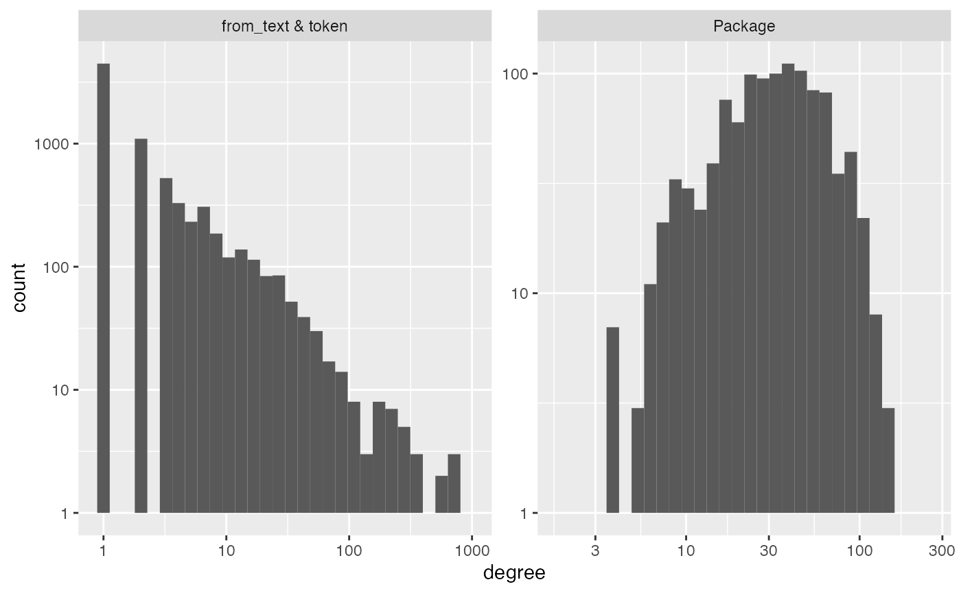
#> # A tibble: 6 × 3
#>   measurement     Package `from_text & token`
#>   <chr>             <dbl>               <dbl>
#> 1 number_of_items    1094                7878
#> 2 average_degree       38                   5
#> 3 median_degree        33                   1
#> 4 percent_le_1          0                  57
#> 5 percent_le_2          0                  71
#> 6 percent_le_3          0                  77
im_text$column_universe |> arrange(desc(n))
#> # A tibble: 7,878 × 4
#>    from_text   token         n col_num
#>    <chr>       <chr>     <int>   <int>
#>  1 Description and        2571       1
#>  2 Description the        1999       2
#>  3 Description of         1388       3
#>  4 Description for        1350       4
#>  5 Description to         1104       5
#>  6 Description a          1013       6
#>  7 Description in          722       7
#>  8 Description functions   581       8
#>  9 Description data        541       9
#> 10 Description package     515      10
#> # ℹ 7,868 more rows
Here we see the stopwords. These will form high degree nodes in your
interaction_model graph. A factor that loads heavily on
these is often a factor that indicates “document length”. Alternatively,
you can remove stop words like this:
# remove stop words by removing them from the column_universe,
#  then use the function subset_im to renumber the columns/rows and remove any lines from interaction_tibble
im_text$column_universe = im_text$column_universe |>
  anti_join(tidytext::stop_words, by = c("token"="word"))
im_text = im_text |> subset_im()
# inspect the new column_universe to see that the stop words have been removed.
im_text$column_universe |> arrange(desc(n))
#> # A tibble: 7,435 × 4
#>    from_text   token         n col_num
#>    <chr>       <chr>     <int>   <int>
#>  1 Description functions   581       1
#>  2 Description data        541       2
#>  3 Description package     515       3
#>  4 Description models      319       4
#>  5 Description doi         285       5
#>  6 Description methods     226       6
#>  7 Description analysis    218       7
#>  8 Description function    164       8
#>  9 Description model       155       9
#> 10 Description based       142      10
#> # ℹ 7,425 more rows
You can also parse multiple columns with the &:
im_imports_authors = make_interaction_model(top_packages, ~Package*(Imports&Author&Description&Title), parse_text = TRUE)
im_imports_authors$row_universe
#> # A tibble: 1,094 × 3
#>    Package             n row_num
#>    <chr>           <int>   <int>
#>  1 broom             671       1
#>  2 DescTools         562       2
#>  3 ff                488       3
#>  4 knitr             430       4
#>  5 ape               411       5
#>  6 spatstat          392       6
#>  7 spdep             381       7
#>  8 netmeta           346       8
#>  9 Seurat            339       9
#> 10 spatstat.linnet   333      10
#> # ℹ 1,084 more rows
im_imports_authors$column_universe
#> # A tibble: 17,696 × 4
#>    from_text   token         n col_num
#>    <chr>       <chr>     <int>   <int>
#>  1 Author      ctb        2744       1
#>  2 Description and        2571       2
#>  3 Author      aut        2077       3
#>  4 Description the        1999       4
#>  5 Description of         1388       5
#>  6 Description for        1350       6
#>  7 Description to         1104       7
#>  8 Author      https      1048       8
#>  9 Description a          1013       9
#> 10 Author      orcid.org  1008      10
#> # ℹ 17,686 more rows
So, let’s do a quick analysis. We see that the tokens are very very
sparse, with 64% of tokens appearing only once! We will want to keep an
eye out for localization in the streaks plot.
diagnose(im_imports_authors)
#> Warning in scale_y_log10(): log-10 transformation introduced
#> infinite values.
#> Warning: Removed 5 rows containing missing values or values outside the scale range
#> (`geom_bar()`).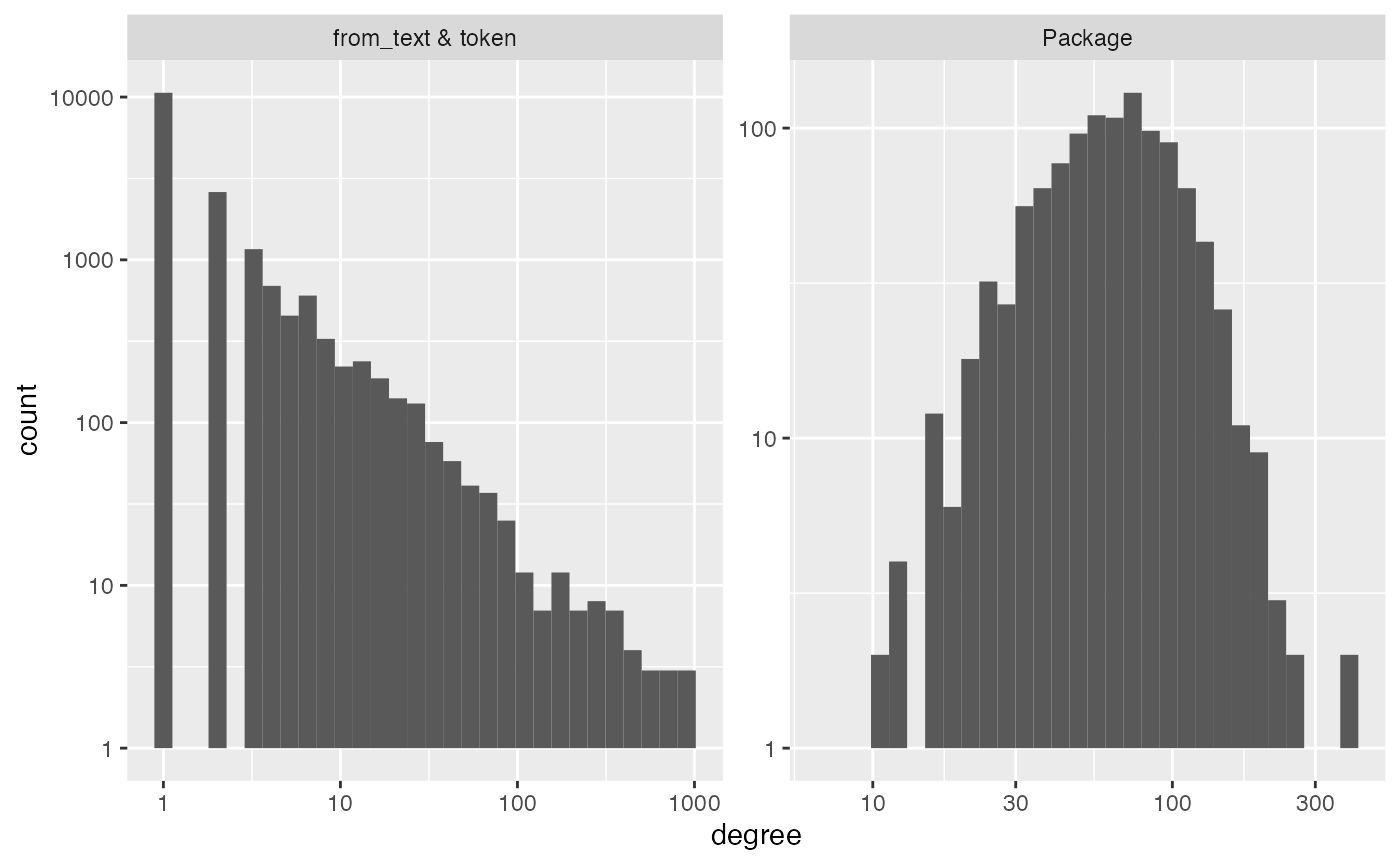
#> # A tibble: 6 × 3
#>   measurement     Package `from_text & token`
#>   <chr>             <dbl>               <dbl>
#> 1 number_of_items    1094               17696
#> 2 average_degree       70                   4
#> 3 median_degree        62                   1
#> 4 percent_le_1          0                  60
#> 5 percent_le_2          0                  75
#> 6 percent_le_3          0                  81
Because it is so sparse, the function core can be used
to pull out the densely connected core of the data. In particular, it
treats the interaction_model object as a bipartite graph,
then finds the k-core of the largest connected
component.
# you can remove these words that appear less than 5 times (and documents that have less than 5 words) via:
im_text = core(im_text, core_threshold = 5)
#> [1] "adding graph summaries (coreness and connected components)."
diagnose(im_text)
#> Warning in scale_y_log10(): log-10 transformation introduced
#> infinite values.
#> Warning: Removed 8 rows containing missing values or values outside the scale range
#> (`geom_bar()`).
#> # A tibble: 6 × 3
#>   measurement     Package `from_text & token`
#>   <chr>             <dbl>               <dbl>
#> 1 number_of_items    1002                1188
#> 2 average_degree       18                  15
#> 3 median_degree        15                   9
#> 4 percent_le_1          0                   0
#> 5 percent_le_2          0                   0
#> 6 percent_le_3          0                   0
We can identify the largest statistically reasonable choice for
k using pick_dim which uses cross-validated eigenvalues
as implimented in the package gdim (github).

eigcv
#> Estimated graph dimension:    20
#>
#> Number of bootstraps:         20
#> Edge splitting probabaility:  0.1
#> Significance level:       0.05
#>
#>  ------------ Summary of Tests ------------
#>   k         z        pvals         padj
#>   1 52.485295 0.000000e+00 0.000000e+00
#>   2 11.238153 1.324323e-29 1.324323e-29
#>   3  6.928938 2.120063e-12 2.120063e-12
#>   4 18.267156 7.556182e-75 7.556182e-75
#>   5 11.858499 9.721468e-33 9.721468e-33
#>   6  5.716077 5.450576e-09 5.450576e-09
#>   7  5.689208 6.381499e-09 6.381499e-09
#>   8  7.313266 1.303634e-13 1.303634e-13
#>   9  7.949433 9.368327e-16 9.368327e-16
#>  10  9.502129 1.028216e-21 1.028216e-21
#>  11  9.000204 1.126495e-19 1.126495e-19
#>  12  6.834819 4.105421e-12 4.105421e-12
#>  13  4.717907 1.191416e-06 1.191416e-06
#>  14  6.710736 9.682262e-12 9.682262e-12
#>  15  7.593119 1.561483e-14 1.561483e-14
#>  16  8.220860 1.010248e-16 1.010248e-16
#>  17  8.542267 6.580719e-18 6.580719e-18
#>  18  8.822639 5.589641e-19 5.589641e-19
#>  19  8.112027 2.489107e-16 2.489107e-16
#>  20  7.331145 1.140971e-13 1.140971e-13
I’m going to pick 10 for convenience.
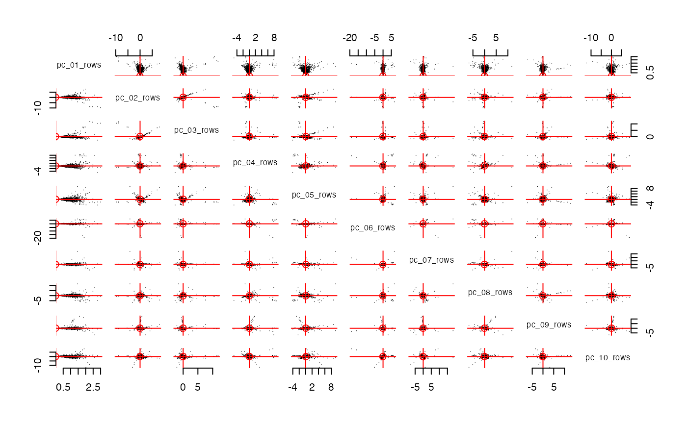
streaks(pcs, "columns")
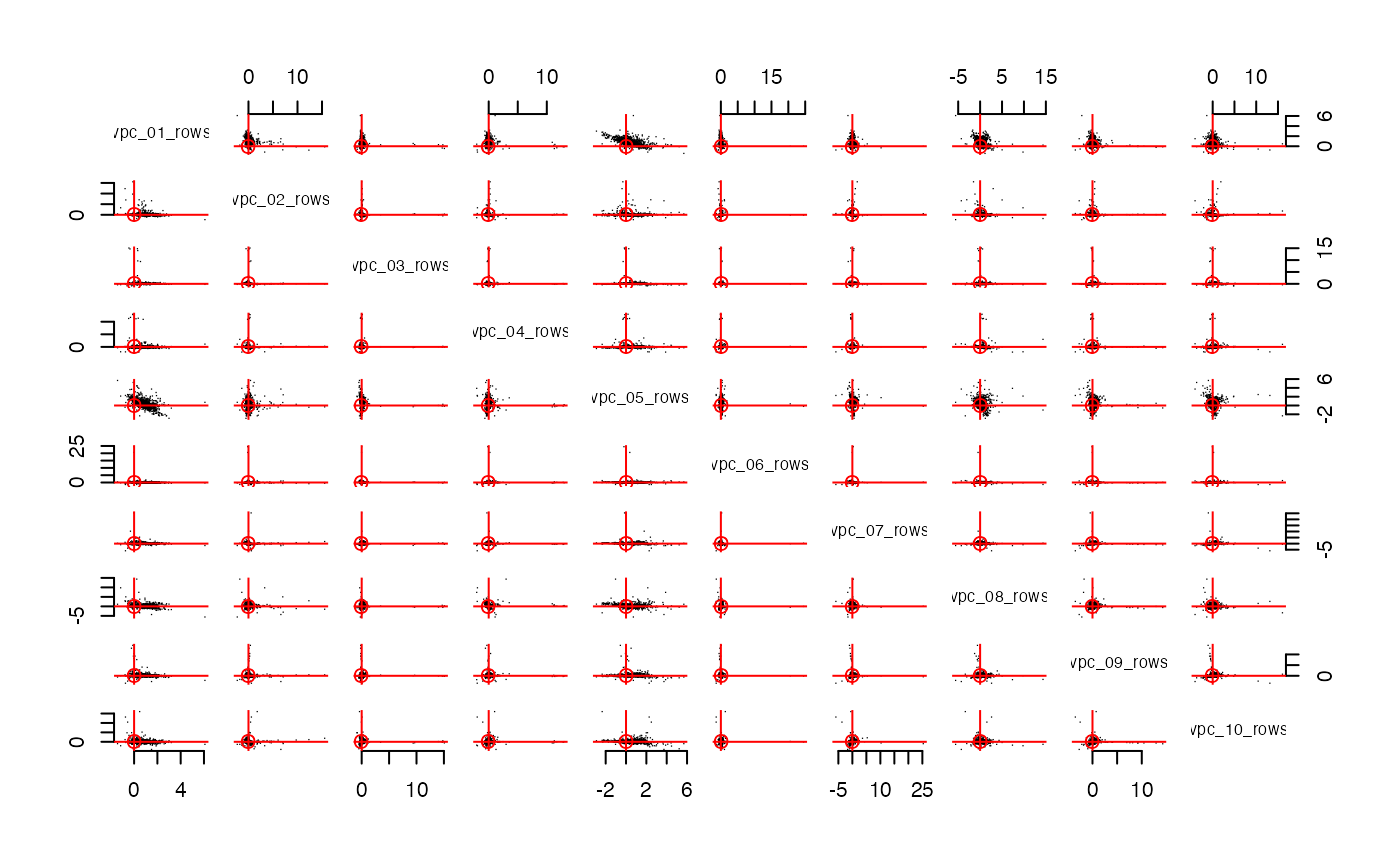
streaks(spcs, "columns")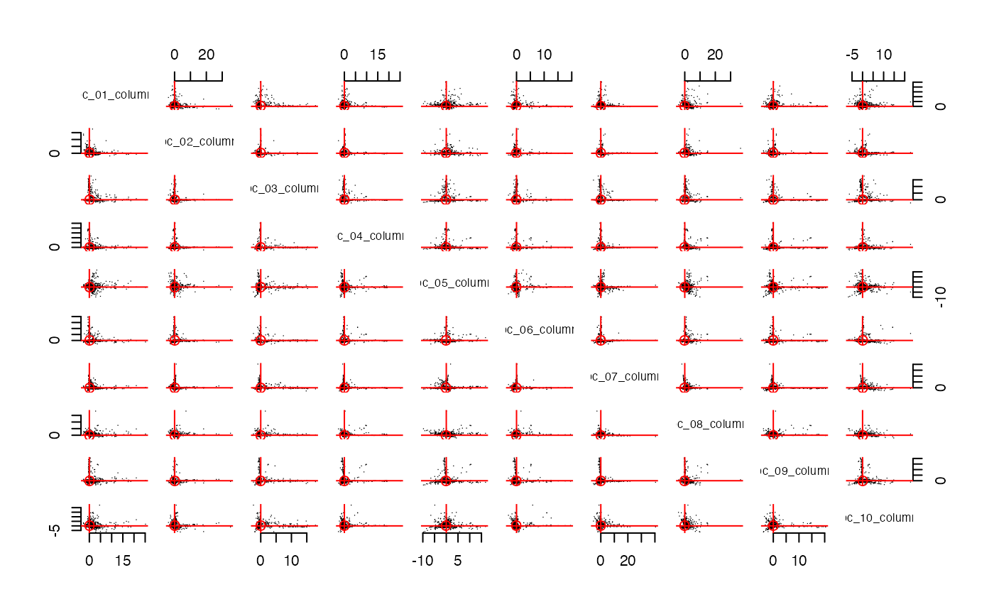
Let’s use
im = make_interaction_model(all_packages, ~Package*Imports, parse_text = TRUE, to_lower = FALSE)
pcs = im |> core() |> pca(10)
#> [1] "adding graph summaries (coreness and connected components)."
im_text = make_interaction_model(top_packages, ~Package*(Title & Description), parse_text= TRUE)
im_text$column_universe = im_text$column_universe |> dplyr::anti_join(tidytext::stop_words, by = c("token"="word"))
im_text = im_text |> subset_im() |> core()
#> [1] "adding graph summaries (coreness and connected components)."
bff(pcs, im_text, num_best = 4)
#> # A tibble: 0 × 1
#> # ℹ 1 variable: factor <chr>