STAT340: Discussion 5: Hypothesis Testing

Just for fun (1 min)

Correlation doesn't imply causation, but it does waggle its eyebrows suggestively and gesture furtively while mouthing 'look over there'.

Group Discussion (5-10 min)

As a group, briefly discuss the following questions!

What is the the difference between the null and alternative hypotheses?
- Don’t just say “we assume the null”; why do we usually choose "mean = __" or “no effect” as the null rather than as the alternative? Hint: think about our ability to predict the outcome and compute \(p\)-values. Is this equally easy to do under both hypotheses?
Why do we use \(\leq\) and \(\geq\) instead of \(=\) in for example \(\small P(X\geq9)\)? How does this relate to the idea of a “surprising set”?

Exercise (rest of time)

Now, break off into groups of 3-4 students. In your group, nominate one person to share their screen.

This week, there is just one exercise with 7 parts. There is a lot of writing to help guide you through the parts. Please make sure you read everything carefully and understand the reasoning behind each step before proceeding onto the next step.

Background

In other courses, you’ve seen the sample mean being used to construct a statistic (e.g. \(z\) or \(t\) value) that is used to test a hypothesis. Last week, you’ve also seen the longest run being used as a statistic to test a hypothesis.

There is nothing special about these two examples, and in general you can use any property of a sample to construct a statistic to test a hypothesis, as long as that property would be observably different under the null and alternative hypotheses. (e.g. the proportion of heads AND the longest run length BOTH depend on the fairness of the coin and whether someone faked the sequence).

Sometimes, these statistics are either not applicable or not sufficient, and you may need to construct other test statistics to test a hypothesis. For this exercise, we will explore yet another way you can test a hypothesis.

Setup

A certain professional basketball player believes he has “hot hands”, especially when shooting 3-point shots (i.e. if he makes a shot, he’s more likely to also make the next shot). His friend doesn’t believe him, so they make a wager and hire you, a statistician, to settle the bet.

As a sample, you observe the next morning as the player takes the same 3-point shot 200 times in a row (assume he is well rested and doesn’t get tired during this, so his level of mental focus doesn’t change during the experiment). You obtain the following results, where Y denotes a success and N denotes a miss:

YNNNNYYNNNYNNNYYYNNNNNYNNNNNNNNNYNNNNNYYNYYNNNYNNNNYNNYYYYNNYYNNNNNNNNNNNNNNNYYYNNNYYYYNNNNNYNYYNNNNYNNNNNNYNNNYNNYNNNNNYNYYYNNYYYNYNNNNYNNNNNNNYYNNYYNNNNNNYNNNYNNNNNNNNYNNNYNNNNNYYNNNNNNYYYYYYNYYNNYN

Note that testing to see if he has “hot hands” is equivalent to testing the hypothesis that the previous shot does not affect the next shot (i.e. that his throws are independent) (also, you may assume that it is impossible for him to have the opposite of “hot hands” where making a previous shot makes him more likely to “choke” and miss the next shot).

(a)

State appropriate null and alternative hypotheses for this problem. (Hint: remember, the alternative is usually the effect you’re looking for (e.g. the drug works), and the null is usually the absence thereof.)

\(H_0\): _______________

\(H_a\): _______________

(b)

Run the code below to import the sequence of throws and verify that it’s been saved correctly as a vector of individual shots.

# the sequence of throws is broken up into 4 chunks for readbility, then
# paste0 is used to merge them into a single sequence, then
# strplit("YN...N",split="") is used to split the string at every "", so
# we get a vector of each character, and finally
# [[1]] is used to get the vector itself (strsplit actually outputs a list
# with the vector as the first element; [[1]] removes the list wrapper)
# 
# for more info about the strsplit function, see
# https://www.journaldev.com/43001/strsplit-function-in-r

throws = strsplit(
   paste0("YNNNNYYNNNYNNNYYYNNNNNYNNNNNNNNNYNNNNNYYNYYNNNYNNN",
          "NYNNYYYYNNYYNNNNNNNNNNNNNNNYYYNNNYYYYNNNNNYNYYNNNN",
          "YNNNNNNYNNNYNNYNNNNNYNYYYNNYYYNYNNNNYNNNNNNNYYNNYY",
          "NNNNNNYNNNYNNNNNNNNYNNNYNNNNNYYNNNNNNYYYYYYNYYNNYN"), split="")[[1]]

# DO THIS: uncomment the line below to verify it's been correctly imported
# print(throws)

(c)

Will a binomial-type test like what you did for homework 2 (e.g. \(\scriptsize P(X>...)\)) be useful here for this problem? (Hint: does the binomial-type test care about the order of outcomes?)

REPLACE THIS TEXT WITH RESPONSE

(d)

Since the existence of a “hot hands” effect will tend to increase the runs of successes (and thus also decrease the runs of misses), you can try to use a longest-run-length statistic to reject the hypothesis (because this statistic is distributed differently under the null and alternative hypotheses). However, this test has relatively low power, i.e. it’s not as effective in detecting a “hot hands” effect if it exists (which it does (these throws were carefully generated to contain the effect (but you don’t know this yet!))).

We can show this directly! Under the null hypothesis (if you wrote the correct one), the order of the throws shouldn’t matter. Therefore, we can randomly reorder the sequence of throws and compare the longest run length in these random reordered sequences, or permutations, with the run length of the original sequence. If the original sequence has a very different run length compared to most of the reordered sequences, this would be evidence against the null hypothesis.

(Side note: this is also known as an approximate or Monte Carlo permutation test and is an important technique frequently used in other tests/methods.)

We begin by rewriting the longest-run-length function from discussion 4 and lecture to also accept letters like “Y” and “N” (and in fact any value) when detecting runs.

# modified longest run function that accepts any value (that isn't NA)
longestRun = function(vec){
  return(with(rle(na.fail(vec)),max(c(0,lengths))))
}

Next, write a function that, given a vector vec and a number of replicates n , will do the following:

randomly reorder the elements of the vector to get a permutation
- hint: use the sample function without replacement!
compute the longest run of each randomized vector
- hint: use the longestRun function defined previously!
repeat the above steps n times
- hint: there are fancier optimized ways to do this, but a simple for loop will work!
return a new vector with all the longest-run lengths

# DO THIS: uncomment the function below; this is a template to get you started
# PRO TIP: quickly comment/uncomment lines by selecting the lines and then
#          using CTRL+SHIFT+C on Windows or COMMAND+SHIFT+C on Mac,
#          OR by going to the menu bar and choosing "Code" -> "Comment/Uncomment lines"
# 
# getPermutedRuns = function(vec,n){
#    
#    # pre-allocate vector that will be returned
#    runs = rep(NA,n)
#    
#    # run for loop n times
#    for(i in 1:n){
#       
#       # permute the vector
#       permuted = ...
#       
#       # compute longest run
#       run = ...
#       
#       # save result
#       runs[i] = run
#    }
#    
#    # return results of all permutations
#    return(runs)
# }

(e)

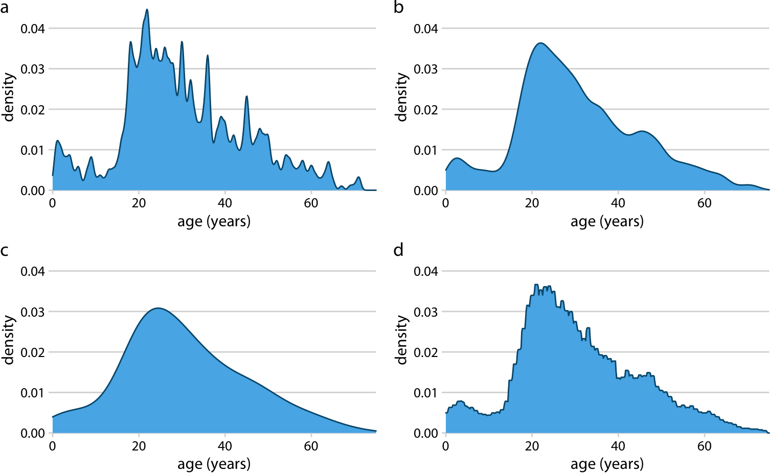
Now, run the function for some large \(n\) (at least 1,000 but can you do 10,000?) and make a density plot of the run lengths of the permuted sequences (if your density plots looks wavy like the top left plot here, you can change the adjust parameter (which controls smoothness) in geom_density like this from 1 to 2 or even higher (try to use the smallest adjust you can that makes the plotted curve look smooth)). Then, add a vertical line on your plot corresponding to the longest run length of the original sequence of throws. You should end up with something like this:

(Hint: to use a vector with ggplot, first turn it into a data.frame (I recommend using a function like enframe( ) from the tibble package.)

# make plot here

How do the longest-run-lengths of the simulated sequences compare with the original sequence? What is your \(p\)-value for this test statistic? What do you conclude about the hypotheses? (Hint: the \(p\)-value in this case is the proportion of the density curve to the right of the vertical line (count how many are greater than the line), and should be roughly between 0.1 and 0.2).

# compute p-value here (make sure to show the result of the computation!)

REPLACE THIS TEXT WITH YOUR REPSONSE

(f)

I (Bi) promise you that a very large “hot hands” effect exists in the data (again, you don’t know this yet!), so clearly the run length test in this case isn’t powerful enough (in other words, it’s not sensitive enough to the underlying effect). However, we can construct a statistic that gives us a much more powerful test!

Consider every pair of consecutive throws and make a table of the outcomes. For example, the first 8 throws in the sequence are YNNNNYYN. Breaking this into consecutive pairs, we have YN, NN, NN, NN, NY, YY, YN. This gives the table:

NN	NY	YN	YY
3	1	2	1

Suppose we do this for the entire sequence of 200 throws (note this gives you 199 pairs). If we divide the number of NY by the number of NN, we get an estimate for how much more likely he is to make the next shot assuming he missed his last shot.

Similarly, we can divide the number of YY by the number of YN to get an estimate for how much more likely he is to make the next shot assuming he scored his last shot.

Now, note that if the “hot hands” effect really exists in the data, then YY/YN should be larger than NY/NN in a large enough sample (if the sample is too small, our estimates would be too imprecise to be useful), and 200 throws should be large enough to hopefully see a significant difference. We use this fact to construct the following test statistic:

\[R=\frac{(\text{# of YY})/(\text{# of YN})}{(\text{# of NY})/(\text{# of NN})}\]

The ratio \(R\) represents, in some sense, how much more likely the player is to make the next shot if he made the previous shot vs if he didn’t make the previous shot (note the vs). In other words, this is exactly the effect of the previous shot on the next shot!

If there is a “hot hands” effect, the numerator should be greater than the denominator and we should have \(R>1\). If the throws are independent and do not affect each other then in theory we should have \(R=1\). If the player is actually a choker and is more likely to miss after a successful shot, we should have \(R<1\). (Side note: this is basically an odds ratio).

To save time, I already wrote a function that splits the sequence of throws into consecutive pairs and then makes a table of the outcomes.

# install the runner package if necessary
if(!"runner" %in% rownames(installed.packages())) install.packages("runner")

# define function for tabulating consecutive pairs
tableOfConsecutivePairs = function(vec){
  return(table(runner::runner(vec,k=2,f=paste,collapse="")[-1]))
}

# test function for correct output
tableOfConsecutivePairs(strsplit("YNNNNYYN",split="")[[1]])

 # 
 # NN NY YN YY 
 #  3  1  2  1


# run function on original sequence of throws
tableOfConsecutivePairs(throws)

 # 
 #  NN  NY  YN  YY 
 # 102  34  35  28

Now, write a function that given the above table as an input, returns the ratio \(R\) as defined above. (Hint: for a given input table tb, you can access, for example, the count of NN with tb["NN"]).

# DO THIS: uncomment the function below and complete it
# 
# getRatioFromTable = function(tb){
#   return(...)
# }
# 
# if you completed the function correctly, the next line should return 2.4
# getRatioFromTable( tableOfConsecutivePairs( throws ) )

Next, modify your simulation loop code from part (d) so that at each step, instead of computing the longest-run-length of each permutation, it computes the ratio \(R\).

# DO THIS: uncomment the function below and complete it
# 
# getPermutedRatios = function(vec,n){
#   ...
#   ...
#   return(...)
# }

(g)

Similar to part (e), run this function \(n\) times (again, at least 1,000 but can you do 10,000?) and plot the density of the result, along with a vertical line marking the ratio of the original sequence. You should end up with something like this:

# run function AND make plot here

Using this test statistic, what is the new \(p\)-value? What do you conclude (i.e. hypothesis decision?) about the basketball player? Does he have hot hands?

# compute p-value here (make sure to show the result of the computation!)

REPLACE THIS TEXT WITH YOUR COMPUTED P-VALUE AND CONCLUSION ABOUT THE PLAYER. DOES HE HAVE “HOT HANDS”?

Submission

As usual, make sure the names of everyone who worked on this with you is included in the header of this document. Then, knit this document and submit both this file and the HTML output on Canvas under Assignments ⇒ Discussion 5

Appendix: Comment about how the throws were generated

As I have explained before, the throws were intentionally generated to have a “hot hands” effect. The first throw was randomly chosen with a \(35\%\) chance of success (chosen based on a quick Google search of average 3-point shot rates). After that, the probability of success of the next shot was dependent on the success of the previous shot. If the previous attempt was a success, this was raised to \(45\%\); if it missed, this was lowered to \(25\%\).

n = 200
throws = rep(NA,n)

for(i in 1:n){
  if(i==1){
    throws[i] = sample(c("Y","N"),1,prob=c(0.35,0.65))
  } else {
    if(throws[i-1]=="Y"){
      throws[i] = sample(c("Y","N"),1,prob=c(0.45,0.55))
    } else{
      throws[i] = sample(c("Y","N"),1,prob=c(0.25,0.75))
    }
  }
}

The numbers were chosen this way so that the average number of 3-point shots made is still close-ish to \(35\%\) (it’s \(31.25\%\) to be exact) and so that the effect is large enough to be detectable, but not so much so that the run-length statistic will also be able to detect an effect (which might happen if the strength of the effect was raised by raising/lowering the numbers even more).

200 was used as the number of throws in the experiment as a balance between lowering the variance of the ratio \(R\) of the generated sequence while still being somewhat plausible for a professional basketball player to achieve.